Lab 2: Conducting a Distance Azimuth Survey

Introduction

On September 19, 2017 my field partner, Anthony Ducosin, and I went out to Putnam Park near the University of Wisconsin Campus and conducted a Tree Survey using Distance and Azimuth. The purpose of this lab is to find the location, type, and circumference of several trees in Putnam Park to practice the Distance Azimuth Method using particular equipment. 

Methods

Data Collection

Anthony and I established two field sites from which we collected data about 10 nearby trees. Data collected included location relative to the field site using distance and azimuth, diameter, and tree type.

Using the GPS Unit shown in Figure 1, we established the site coordinates. It is from these points that all geographic data was collected. The location of the field sites, Site 1 and Site 2, are shown in Map 1. Their coordinates are (44.796047N, 91.501241E) and (44.795523N, 91.500121E), respectively.

Figure 1: GPS Unit

Map 1: Site Locations

We used distance and azimuth to find the positions of 10 trees relative to our site locations. Distance was measured with the laser distance finder shown in Figure 2. Azimuth was measured with a Geographer's Compass pictured in Figure 3. It should be noted that values of the compass are measured by an angle, 0-90 degrees, and a cardinal direction NW, NW, SW, or SE. The values are not in degrees 0-360, and the cardinal direction for each measurement is a necessary piece of data to collect.

Figure 2: Laser Distance Finder

Figure 3: Geographer's Compass

We also collected the diameter of each tree by finding its circumference in the field using the tape measure pictured in figure 4. The value collected was later converted to diameter in excel.

Figure 4: Tape Measure

Neither Anthony nor myself are biologists, so collecting information about they type of tree was rather challenging. We were confident in the fact that all trees measured were deciduous, but we only recorded a data more specific that that when professor Hupy walked by and told us about the tree we were identifying. 

In the field, all data was collected by hand in a notebook. We created a spreadsheet using that data once we got to the lab. The Excel spreadsheet is pictured in Figure 5. When entering longitude, be sure to include a negative sign reflecting that the value is east of the prime meridian, unless you want the data to show up in Mongolia. Azimuth is converted from a 0-90 degree value and direction designation to a 0-360 degree value. The diameter column is populated by Diameter = Circumference / Pi. 

Figure 5: Excel Data Sheet

Map Production

The data from the spreadsheet in Figure 5 was used to make a series of maps. I brought the data into a new file geodatabase as a table. Using the search window, I found Bearing Distance to Line tool, see Figure 6 for more details about this tool. See table 1 for a list of values I entered when using this tool. Any field not explicitly noted I left as default. The results of using this tool is shown in Map 2.

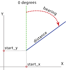Figure 6: Bearing Distance to Line Tool

Creates a new feature class containing geodetic line features constructed based on the values in an x-coordinate field, y-coordinate field, bearing field, and distance field of a table (Source 1).

Table 1: Bearing Distance to Line Tool
In_Table	Excel table (Figure 5)
Out_Featureclass	Tree_dist_as
X_field	Longitude
Y_field	Latitude
Distance_field	Distance
Distance_units	Meters
Bearing_field	Azimuth
Bearing_units	Degrees

Map 2: Result of Bearing Distance to Line Tool

Next, I used the search window to find the Feature Vertices to Points tool, which creates a point feature class "containing points generated from specified vertices or locations of the input features" (Source 2). For Point_Location, I used "all" which is incorrect. I should have used "end" so that the Site position was not included in the final feature class. The result of this tool is shown in Map 3.

Map 3: Result of Feature Vertices to Points Tool

The final step was to symbolize the data so that the tree locations represented tree type and trunk circumference. The results of this are Map 4 and Map 5.

Results

Map 4: Data classified by type of tree

Map 5: Data classified by circumference of tree

Discussion

The Point-Quarter sampling method (Source 3) collects data in a way very similar to how Anthony and I collected our data for this lab. However, we collected the specific geographic location of each of 10 trees by using azimuth and distance. We did not discriminate against quadrant when selecting trees. The method described in Source three picks the 1 closest tree in each of 4 directions to collect data on and does not measure geographic position. Using our method would allow biologists to map out sections of forests, collect more data, and select the four closest trees to measure, rather than the 1 closest in each of 4 directions.

The method described in this lab is excellent for collecting data about features that do not move. This method measuring the position of an object with reference to another, using a wide range of tools, has been used for ages by land surveyors, geographers, and astronomers alike.

With the advent of GPS units, which are increasingly precise and accurate, GPS is the favored method of collecting geospatial data. However, when that technology fails, for whatever reason, collecting data with distance and azimuth is still an option. The distance-azimuth method laid the groundwork for GPS, which uses control points - survey markers measured off one-another and the stars.

Sources

1. http://pro.arcgis.com/en/pro-app/tool-reference/data-management/bearing-distance-to-line.htm
2. http://pro.arcgis.com/en/pro-app/tool-reference/data-management/feature-vertices-to-points.htm
3. http://www.saddleback.edu/faculty/steh/bio3afolder/Point-Quarter%20Lab.pdf